
How big is my dog going to get? A regression analysis with R
The dog on the left is named Maya. She is a labrador retriever (field line), weighs 18 kilograms and is currently eight months old. My girlfriend and I carry the dog several times a day high in the fourth floor. We have learned that is important in the first year. Ok, but how much weight she will increase over the next months? I think: a great question to improve my skills in non-linear regression analysis!
We weigh our dog regularly on our Withings WiFi Body Scale. The data is here:
mydog <- read.csv("https://holtmeier.de/public/maya.csv")
mydog$DATE <- as.Date(mydog$DATE, "%Y/%m/%d")
mydog$AGE <- as.numeric(mydog$DATE - as.Date("2011-05-04"))
In line 3, I calculate the days since birth, because my approach does not work with dates. At least I do not know how. Basically, I know little to nothing about growth models of dogs. Therefore, I approach the question quite naive. I make two assumptions:
- The growth is non-linear. It is negative exponential, as it is in this example.
- The weight asymptotically approaches a genetically predetermined maximum value.
I have found the function SSasymp in „stats“ package. The description says: „This self start model Evaluate the asymptotic regression function and its gradient It has an initial attribute that will evaluate initial estimates of the parameters Asym, R0, and lrc for a given set of data..“ This is what I was looking for.
[sourcecode language=“r“]
require(stats)
fm <- nls(WEIGHT ~ SSasymp(AGE, Asym, R0, lrc), data = mydog)
summary(fm)
[/sourcecode]
The code results in the following output:
Formula: WEIGHT ~ SSasymp(AGE, Asym, R0, lrc)

Parameters:
     Estimate Std. Error t value Pr(>|t|)
Asym 22.92878    0.74010  30.981  < 2e-16 ***
R0   -2.59439    0.52484  -4.943 8.71e-06 ***
lrc  -5.07800    0.07263 -69.912  < 2e-16 ***
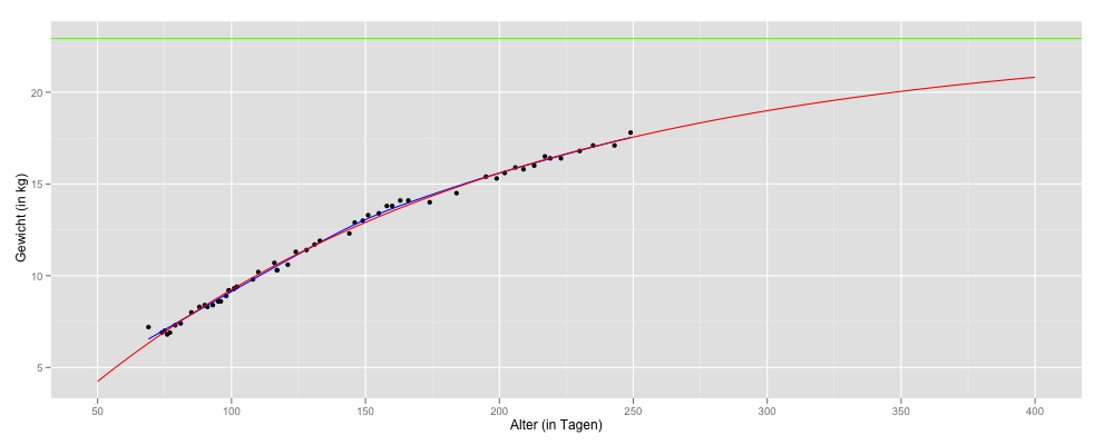
22.92878 is the numeric parameter representing the horizontal asymptote on the right side (very large values of input). So this is the estimate of the target weight for our dog (line 6, green line). Finally, I would like to visualize my data, including the regression curve. I use ggplot2 – as usual. In addition to model-based curve (line 5, red curve), I draw the model-free spline fit (line 4, blue curve). A spline fit per se does not assume a functional relationship between time and growth data (Kahm, M. et al. al., 2010).
require(ggplot2)
ggplot(data=mydog, aes(x=AGE, y=WEIGHT)) +
geom_point() +
geom_smooth(color="Blue", se=F) +
geom_smooth(method="nls", formula=y~SSasymp(x, Asym, R0, lrc), color="red", se=F, fullrange=T) +
geom_hline(color="green", yintercept=22.92878) +
scale_x_continuous(limits=c(50,400)) +
xlab("Alter (in Tagen)") + ylab("Gewicht (in kg)")
As I said, I am still learning. Are there better ways to estimate the weight of my dog? Other models (eg the Gompertz growth function)? I am looking forward to improving information!