Reflect your Personnel Selection: R & Taylor-Russell Tables

Taylor-Russell tables (Taylor & Russell, 1939) are designed to estimate the percentage of future employees who will be successful on the job if a particular selection method (eg. test, assessment center, interview) is used. I have already described the our Taylor-Russell-Tool (in German).

Now I will show how the number of recruited candidates is calculated precisely with R. I use the manipulate package. Therefore, the code will only run in the RSudio IDE. The big advantage is that one can easily observe the influences of

the base rate of potentially suitable persons in the non-selected group of applicants as well as
the validity of the selection process (by moving the slider).

This little program is excellent for teaching.

The calculations are based on an article of Richard A. Mclellan in the journal „Personnel Decisions International“ (1999): Theoretical Expectancies: Replacing Classic Utility Tables with Flexible, Accurate Computing Procedures.

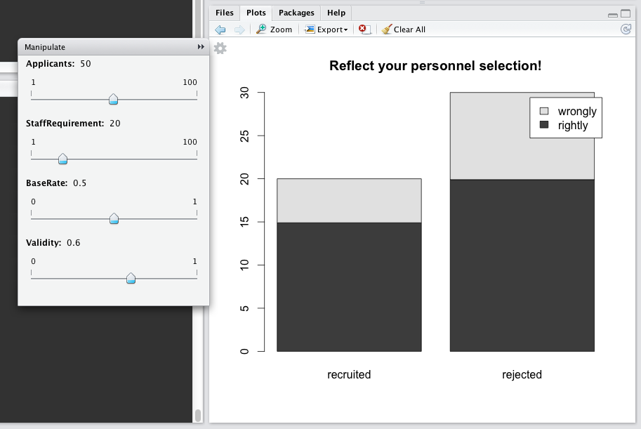
And this is the result. Have fun trying.

F1 <- function(P) { SPLIT <- 0.42 A0 <- 2.50662823884 A1 <- -18.61500062529 A2 <- 41.391199773534 A3 <- -25.44106049637 B1 <- -8.4735109309 B2 <- 23.08336743743 B3 <- -21.06224101826 B4 <- 3.13082909833 C0 <- -2.78718931138 C1 <- -2.29796479134 C2 <- 4.85014127135 C3 <- 2.32121276858 D1 <- 3.54388924762 D2 <- 1.63706781897 Q <- P - 0.5 if (abs(Q) <= SPLIT) { R <- Q*Q PPN <- Q * (((A3 * R + A2) * R + A1) * R + A0) / ((((B4 * R + B3) * R + B2) * R + B1)*R +1.0) return(PPN) } R <- P if (Q > 0) {R =1.0-P} if (R <= 0) { print("You have entered a value that is not permitted. The result is false.") return(0) } R <- sqrt(-log(R)) PPN <- (((C3 * R + C2) * R + C1) * R + C0) / ((D2 * R + D1) * R + 1.0) if (Q < 0) {PPN =-PPN} return(PPN) } F2 <- function(X) { P1A <- 242.667955230532 P1B <- 21.97926616182942 P1C <- 6.996383488661914 P1D <- -3.5609843701815E-02 Q1A <- 215.058875869861 Q1B <- 91.1649054045149 Q1C <- 15.0827976304078 Q1D <- 1.0 P2A <- 300.459261020162 P2B <- 451.918953711873 P2C <- 339.320816734344 P2D <- 152.98928504694 P2E <- 43.1622272220567 P2F <- 7.21175825088309 P2G <- .564195517478994 P2H <- -1.36864857382717E-07 Q2A <- 300.459260956983 Q2B <- 790.950925327898 Q2C <- 931.35409485061 Q2D <- 638.980264465631 Q2E <- 277.585444743988 Q2F <- 77.0001529352295 Q2G <- 12.7827273196294 Q2H <- 1.0 P3A <- -2.99610707703542E-03 P3B <- -4.94730910623251E-02 P3C <- -.226956593539687 P3D <- -.278661308609648 P3E <- -2.23192459734185E-02 Q3A <- 1.06209230528468E-02 Q3B <- .19130892610783 Q3C <- 1.05167510706793 Q3D <- 1.98733201817135 Q3E <- 1.0 SQRT2 <- 1.4142135623731 SQRTPI <- 1.77245385090552 Y <- X/SQRT2 if (Y < 0) { Y <- -Y SN <- -1.0 } else { SN <- 1.0 } Y2 <- Y * Y if (Y < 0.46875) { R1 <- ((P1D * Y2 + P1C) * Y2 + P1B) * Y2 + P1A R2 <- ((Q1D * Y2 + Q1C) * Y2 + Q1B) * Y2 + Q1A ERFVAL <- Y * R1 / R2 if (SN == 1) LOAREA <- 0.5 + 0.5 * ERFVAL else LOAREA <- 0.5 - 0.5 * ERFVAL } else { if (Y < 4.0) { R1 <- ((((((P2H * Y + P2G) * Y + P2F) * Y + P2E) * Y + P2D) * Y + P2C) * Y + P2B) * Y + P2A R2 <- ((((((Q2H * Y + Q2G) * Y + Q2F) * Y + Q2E) * Y + Q2D) * Y + Q2C) * Y + Q2B) * Y + Q2A ERFCVAL <- exp(-Y2) * R1 / R2 } else { Z <- Y2 * Y2 R1 <- (((P3E * Z + P3D) * Z + P3C) * Z + P3B) * Z + P3A R2 <- (((Q3E * Z + Q3D) * Z + Q3C) * Z + Q3B) * Z + Q3A ERFCVAL <- (exp(-Y2) / Y) * (1.0 / SQRTPI + R1 / (R2 * Y2)) } if (SN == 1) LOAREA <- 1.0 - 0.5 * ERFCVAL else LOAREA <- 0.5 * ERFCVAL } UPAREA <- 1.0 - LOAREA return(UPAREA) } F3 <- function(H1, HK, R) { X <- c(0.04691008, 0.23076534, 0.5, 0.76923466, 0.95308992) W <- c(0.018854042, 0.038088059, 0.0452707394, 0.038088059, 0.018854042) H2 <- HK H12 <- (H1*H1 + H2*H2)/2.0 BV <- 0 if (abs(R) >= 0.7) { R2 <- 1.0-R*R R3 <- sqrt(R2) if (R < 0) H2 <- -H2 H3 <- H1*H2 H7 <- exp(-H3 / 2.0) if (R2 != 0) { H6 <- abs(H1 - H2) H5 <- H6 * H6 / 2.0 H6 <- H6 / R3 AA <- 0.5 - (H3 / 8.0) AB <- 3.0 - (2.0 * AA * H5) BV <- 0.13298076 * H6 * AB * F2(H6) - exp(-H5 / R2) * (AB + AA * R2) * 0.053051647 for (i in 1:5) { R1 <- R3 * X[i] RR <- R1 * R1 R2 <- sqrt( 1.0- RR) BV <- BV - W[i] * exp(-H5 / RR) * (exp(-H3 / (1.0 + R2)) / R2 / H7 - 1.0 - AA * RR) } } if (R > 0 & H1 > H2) { BV <- BV * R3 * H7 + F2(H1) return(BV) } if (R > 0 & H1 <= H2) { BV <- BV * R3 * H7 + F2(H2) return(BV) } if (R < 0 & (F2(H1) - F2(H2)) < 0) { BV <- 0 - BV * R3 * H7 return(BV) } if (R < 0 & (F2(H1) - F2(H2)) >= 0) { BV <- (F2(H1) - F2(H2)) - BV * R3 * H7 return(BV) } } H3 <- H1 * H2 for (i in 1:5) { R1 <- R * X[i] RR2 <- 1.0 - R1 * R1 BV <- BV + W[i] * exp((R1 * H3 - H12) / RR2) / sqrt(RR2) } BV <- F2(H1) * F2(H2) + R * BV return(BV) } true_positives <- function(N, ToSelect,BaseRate, Validity) {round(F3(F1(1.0-ToSelect/N), F1(1.0-BaseRate), Validity)/(ToSelect/N)*ToSelect,1)} false_positives <- function(N, ToSelect,BaseRate, Validity) {round(ToSelect-F3(F1(1.0-ToSelect/N), F1(1.0-BaseRate), Validity)/(ToSelect/N)*ToSelect,1)} false_negatives <- function(N, ToSelect,BaseRate, Validity) {round(N*BaseRate - F3(F1(1.0-ToSelect/N), F1(1.0-BaseRate), Validity)/(ToSelect/N)*ToSelect,1)} true_negatives <- function(N, ToSelect,BaseRate, Validity) {N - true_positives(N, ToSelect,BaseRate, Validity) - false_positives(N, ToSelect,BaseRate, Validity) - false_negatives(N, ToSelect,BaseRate, Validity)} library(manipulate) manipulate( barplot( matrix(c(true_positives(Applicants, StaffRequirement, BaseRate, Validity), false_positives(Applicants, StaffRequirement, BaseRate, Validity), true_negatives(Applicants, StaffRequirement, BaseRate, Validity), false_negatives(Applicants, StaffRequirement, BaseRate, Validity)), nrow = 2, ncol=2, byrow=FALSE, dimnames = list(c("rightly", "wrongly"), c("recruited", "rejected"))), legend.text=TRUE, main="Reflect your personnel selection!"), Applicants=slider(1,100, step=1, initial = 50), StaffRequirement=slider(1,100, step=1, initial = 10), BaseRate=slider(0,1, step=.01, initial = .25), Validity=slider(0,1, step=.01, initial = .37))

3 comments

Eamonn
Februar 17, 2012 Antworten

Very nice – hadn’t seen / used the manipulate package before!
Sergei Petrov
Februar 19, 2012 Antworten

> X R for (i in 1:5) { R1 R1
[1] 9.530899

for() not needed?
- Stephan
  Februar 19, 2012 Antworten
  
  Hi Sergei,
  which line do you mean?